41 data labels excel chart
Understanding Excel Chart Data Series, Data Points, and Data ... Sep 19, 2020 · Charts and graphs in Excel and Google Sheets use data points, data markers, and data labels to visualize data and convey information. If you want to create powerful charts, learn how each of these elements works and how to use them properly. Chart.ApplyDataLabels method (Excel) | Microsoft Docs The type of data label to apply. True to show the legend key next to the point. The default value is False. True if the object automatically generates appropriate text based on content. For the Chart and Series objects, True if the series has leader lines. Pass a Boolean value to enable or disable the series name for the data label.
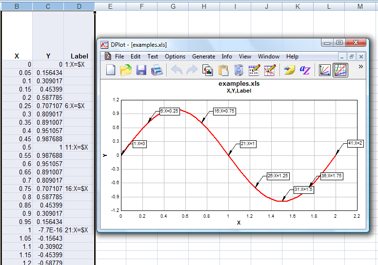
Prevent Overlapping Data Labels in Excel Charts - Peltier Tech May 24, 2021 · Here is the chart after running the routine, without allowing any overlap between labels (OverlapTolerance = zero).All labels can be read, but the space between them is greater than needed (you could almost stick another label between any two adjacent labels here), and some labels have moved far from the points they label.
Data labels excel chart
Excel Charts - Aesthetic Data Labels - Tutorials Point To place the data labels in the chart, follow the steps given below. Step 1 − Click the chart and then click chart elements. Step 2 − Select Data Labels. Click to see the options available for placing the data labels. Step 3 − Click Center to place the data labels at the center of the bubbles. Format a Single Data Label How to Add Data Labels in Excel - Excelchat | Excelchat After inserting a chart in Excel 2010 and earlier versions we need to do the followings to add data labels to the chart; Click inside the chart area to display the Chart Tools. Figure 2. Chart Tools Click on Layout tab of the Chart Tools. In Labels group, click on Data Labels and select the position to add labels to the chart. Figure 3. How to Add Labels to Scatterplot Points in Excel - Statology Next, click anywhere on the chart until a green plus (+) sign appears in the top right corner. Then click Data Labels, then click More Options… In the Format Data Labels window that appears on the right of the screen, uncheck the box next to Y Value and check the box next to Value From Cells.
Data labels excel chart. Move data labels - support.microsoft.com Click any data label once to select all of them, or double-click a specific data label you want to move. Right-click the selection > Chart Elements > Data Labels arrow, and select the placement option you want. Different options are available for different chart types. How to use cell values for excel chart labels - How to We want to chart the sales values and use the change values for data labels. Use Cell Values for Chart Data Labels. Select range A1:B6 and click Insert > Insert Column or Bar Chart > Clustered Column. The column chart will appear. We want to add data labels to show the change in value for each product compared to last month. Select the chart ... Change the format of data labels in a chart To get there, after adding your data labels, select the data label to format, and then click Chart Elements > Data Labels > More Options. To go to the appropriate area, click one of the four icons ( Fill & Line, Effects, Size & Properties ( Layout & Properties in Outlook or Word), or Label Options) shown here. Edit titles or data labels in a chart - support.microsoft.com On a chart, click one time or two times on the data label that you want to link to a corresponding worksheet cell. The first click selects the data labels for the whole data series, and the second click selects the individual data label. Right-click the data label, and then click Format Data Label or Format Data Labels.
Create Dynamic Chart Data Labels with Slicers - Excel Campus Feb 10, 2016 · Typically a chart will display data labels based on the underlying source data for the chart. In Excel 2013 a new feature called “Value from Cells” was introduced. This feature allows us to specify the a range that we want to use for the labels. Since our data labels will change between a currency ($) and percentage (%) formats, we need a ... How to add data labels from different column in an Excel chart? This method will guide you to manually add a data label from a cell of different column at a time in an Excel chart. 1.Right click the data series in the chart, and select Add Data Labels > Add Data Labels from the context menu to add data labels. Excel Chart Data Labels-Modifying Orientation - Microsoft Community In reply to PaulaAB's post on September 13, 2016. Hi Paula, You can right click on the data label part then select Format Axis. Click on the Size & Properties tab then adjust the Text Direction or Custom Angle. Thanks, How to add text labels on Excel scatter chart axis - Data Cornering By default, you can not add text labels on Excel scatter chart axis, but here is a workaround that allows you to do that. You can change Excel scatter chart horizontal or vertical axis labels using a dummy series. Here is how to do that in a few simple steps. Here is the data that I would like to display in the Excel scatter chart. In addition ...
Add data labels and callouts to charts in Excel 365 | EasyTweaks.com Excel also gives you the option of formatting the data labels to suit your desired look if you don't like the default. To make changes to the data labels, right-click within the chart and select the "Format Labels" option. Some of the formatting options you will have include; changing the label position, changing its alignment angle, and many more. Add a DATA LABEL to ONE POINT on a chart in Excel Click on the chart line to add the data point to. All the data points will be highlighted. Click again on the single point that you want to add a data label to. Right-click and select ' Add data label ' This is the key step! Right-click again on the data point itself (not the label) and select ' Format data label '. Add or remove data labels in a chart - support.microsoft.com Click the data series or chart. To label one data point, after clicking the series, click that data point. In the upper right corner, next to the chart, click Add Chart Element > Data Labels. To change the location, click the arrow, and choose an option. If you want to show your data label inside a text bubble shape, click Data Callout. Custom Chart Data Labels In Excel With Formulas Follow the steps below to create the custom data labels. Select the chart label you want to change. In the formula-bar hit = (equals), select the cell reference containing your chart label's data. In this case, the first label is in cell E2. Finally, repeat for all your chart laebls.
DPlot Windows software for Excel users to create presentation quality ...
How to create Custom Data Labels in Excel Charts Add data labels Create a simple line chart while selecting the first two columns only. Now Add Regular Data Labels. Two ways to do it. Click on the Plus sign next to the chart and choose the Data Labels option. We do NOT want the data to be shown. To customize it, click on the arrow next to Data Labels and choose More Options …
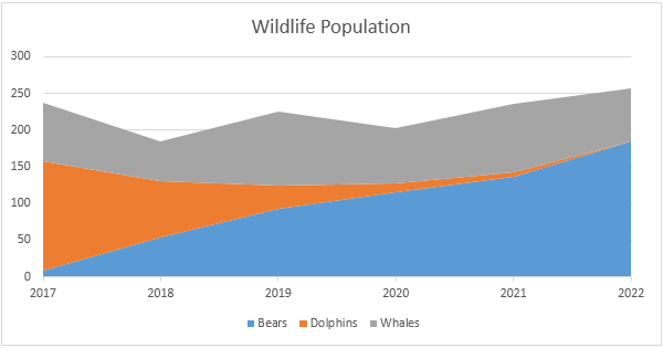
Area Chart in Excel - Easy Excel Tutorial
Add / Move Data Labels in Charts - Excel & Google Sheets We'll start with the same dataset that we went over in Excel to review how to add and move data labels to charts. Add and Move Data Labels in Google Sheets Double Click Chart Select Customize under Chart Editor Select Series 4. Check Data Labels 5. Select which Position to move the data labels in comparison to the bars.

Do My Excel Blog: How to hide the zero percent labels in an Excel pie chart
How to I rotate data labels on a column chart so that they are ... To change the text direction, first of all, please double click on the data label and make sure the data are selected (with a box surrounded like following image). Then on your right panel, the Format Data Labels panel should be opened. Go to Text Options > Text Box > Text direction > Rotate

How to Setup a Pie Chart with no Overlapping Labels | Telerik Reporting
How To Use Dynamic Data Labels To Create Interactive Excel Charts To create a column chart with dynamic data labels, you need to follow these given steps. Select the data & Create a Combo Chart. Now select the column chart for revenue data and a line chart with marker for data labels Add Data Labels to the Line Chart With Marker. After then remove the Line Color and Marker Color.
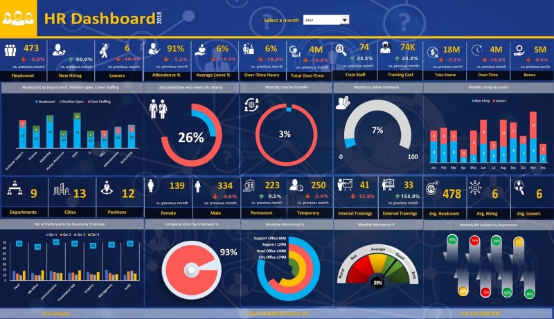
Excel Advanced Dashboard
Excel: How to Create a Bubble Chart with Labels - Statology Step 3: Add Labels. To add labels to the bubble chart, click anywhere on the chart and then click the green plus "+" sign in the top right corner. Then click the arrow next to Data Labels and then click More Options in the dropdown menu: In the panel that appears on the right side of the screen, check the box next to Value From Cells within ...
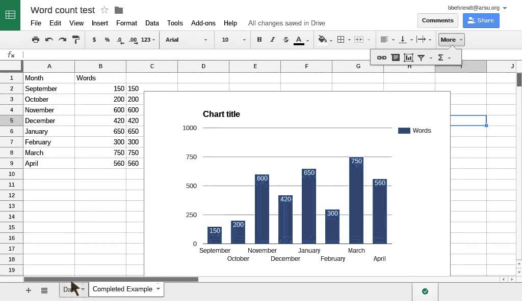
Add labels to a Google chart or graph - YouTube
How to Use Cell Values for Excel Chart Labels Select the chart, choose the "Chart Elements" option, click the "Data Labels" arrow, and then "More Options." Uncheck the "Value" box and check the "Value From Cells" box. Select cells C2:C6 to use for the data label range and then click the "OK" button. The values from these cells are now used for the chart data labels.
10 ways to present variance analysis reports in Excel - PakAccountants.com
How to add total labels to stacked column chart in Excel? 1. Create the stacked column chart. Select the source data, and click Insert > Insert Column or Bar Chart > Stacked Column. 2. Select the stacked column chart, and click Kutools > Charts > Chart Tools > Add Sum Labels to Chart. Then all total labels are added to every data point in the stacked column chart immediately.
Microsoft Excel Tutorials: How to Create a Pie Chart
Excel charts: how to move data labels to legend - Microsoft Tech Community You can't do that, but you can show a data table below the chart instead of data labels: Click anywhere on the chart. On the Design tab of the ribbon (under Chart Tools), in the Chart Layouts group, click Add Chart Element > Data Table > With Legend Keys (or No Legend Keys if you prefer)
Post a Comment for "41 data labels excel chart"