43 excel pivot table column labels

multiple fields as row labels on the same level in pivot table Excel ... multiple fields as row labels on the same level in pivot table Excel 2016. I am using Excel 2016. I have data that lists product models along with relevant data and also production volumes by month. Part of the relevant data are about 5 common part columns with the part # that applies to each model under the appropriate column. Change Blank Labels in a Pivot Table - Contextures Blog You can type any text to replace the (Blank) entry, even a space character, but you can't clear the cell and leave it empty: Select one of the Row or Column Labels that contains the text (blank). Type N/A in the cell, and then press the Enter key. Note: All other (Blank) items in that field will change to display the same text, N/A in this ...

Use column labels from an Excel table as the rows in a Pivot Table Highlight your current table, including the headers; Then from the Data section of the ribbon, select From Table; Highlight all the columns containing data, but not the Year column, and then select Unpivot Columns; Close the dialog and keep the changes. Excel should place the unpivoted data into a new worksheet, looking something like this:

Excel pivot table column labels

Pivot table row labels in separate columns • AuditExcel.co.za Our preference is rather that the pivot tables are shown in tabular form (all columns separated and next to each other). You can do this by changing the report format. So when you click in the Pivot Table and click on the DESIGN tab one of the options is the Report Layout. Click on this and change it to Tabular form. Pivot Table: Pivot table group by custom - Exceljet Once you have the grouping labels in the helper column, add the field directly to the pivot table as a row or column field . Steps. Create a pivot table; Drag the Color field to the Rows area; Drag the Sales field to the Values area; Group items manually. Select items; Right-click and Group; Name group as desired; Repeat for each separate group Centre Column Headings in Excel Pivot Table To centre the column headings in Excel 2007: Select a cell in the pivot table. On the Ribbon, under the PivotTable Tools tab, click Options. At the far left, in the PivotTable group, click Options. On the Layout & Format tab, in the Layout section, add a check mark to Merge and Center Cells With Labels. Click OK.

Excel pivot table column labels. Pivot table - stop it putting 'Column Labels' and 'Row Labels' in Excel Questions. Pivot table - stop it putting 'Column Labels' and 'Row Labels' in. Thread starter Johnny C; Start date Dec 5, 2017; Tags column labels putting row stop ... Pivot Table Banded Columns by Label - MrExcel Message Board sub pivotfrm () dim pt as pivottable, cr as range, db as range, c% set pt = activesheet.pivottables (1) set cr = pt.columnrange set db = pt.databodyrange for c = 1 to cr.columns.count select case cr.cells (1, c) case "jan" ' column label with cr.cells (1, c).resize (db.rows.count).interior .themecolor = xlthemecolordark1 ' gray .tintandshade … How to Use Excel Pivot Table Label Filters In an Excel pivot table, you might want to hide one or more of the items in a Row field or Column field. To do that, you could click the drop down arrow for the Row or Column Labels, to see the list of pivot items in that pivot field. Then, in the list, remove the check mark for items you want to remove. How to make row labels on same line in pivot table? Click any cell in your pivot table, and the PivotTable Tools tab will be displayed. 2. Under the PivotTable Tools tab, click Design > Report Layout > Show in Tabular Form, see screenshot: 3. And now, the row labels in the pivot table have been placed side by side at once, see screenshot:

How to Customize Your Excel Pivot Chart Data Labels - dummies The Data Labels command on the Design tab's Add Chart Element menu in Excel allows you to label data markers with values from your pivot table. When you click the command button, Excel displays a menu with commands corresponding to locations for the data labels: None, Center, Left, Right, Above, and Below. Hide Excel Pivot Table Buttons and Labels To discourage people from changing the pivot table layout, follow these steps to make a couple of changes to the display settings. Right-click any cell in the pivot table; In the pop-up menu, click PivotTable Options; In the PivotTable Options dialog box, click the Display tab; To hide all of the expand/collapse buttons in the pivot table: Pivot Table column label from horizontal to vertical Pivot Table column label from horizontal to vertical After pivot table and with grouping, some column labels have been showed but the caption is on the top. What i want is put the column header at the left of the row as vertical red text show as below. However, i cannot do this, it said "We cant change this part of pivot table". Automatic Row And Column Pivot Table Labels - How To Excel At Excel Hit Pivot Table icon; Next select Pivot Table option; Select a table or range option; Select to put your Table on a New Worksheet or on the current one, for this tutorial select the first option; Click Ok; The Options and Design Tab will appear under the Pivot Table Tool; Select the check boxes next to the fields you want to use to add them to the Pivot Table

Repeat item labels in a PivotTable - support.microsoft.com Right-click the row or column label you want to repeat, and click Field Settings. Click the Layout & Print tab, and check the Repeat item labels box. Make sure Show item labels in tabular form is selected. Notes: When you edit any of the repeated labels, the changes you make are applied to all other cells with the same label. Pivot table column labels • AuditExcel.co.za How to use the Pivot table column labels to construct a meaningful Pivot Table. For updated video clips in structured Excel courses with practical example files, have a look at our MS Excel online training courses . You can even try the Free MS Excel tips and tricks course.; To see if this video matches your skill level (see the suggested skill score below) do our free MS Excel skills assessment. Repeat All Item Labels In An Excel Pivot Table - MyExcelOnline STEP 1: Click in the Pivot Table and choose PivotTable Tools > Options (Excel 2010) or Design (Excel 2013 & 2016) > Report Layouts > Show in Outline/Tabular Form. STEP 2: Now to fill in the empty cells in the Row Labels you need to select PivotTable Tools > Options (Excel 2010) or Design (Excel 2013 & 2016) > Report Layouts > Repeat All Item ... How to Add a Column to a Pivot Table - Excel Tutorials Add a Column to a Pivot Table. Now that we have our data into the Pivot Table, we will put players into the row field and averages of points into the value fields: If you, for whatever reason, wanted a different value (for example, a total sum of points) all you have to do is click the field in values (in this case Average of Points) and select ...

MVP #10: Making a Pivot table that has labels spread across several columns | Productivity Tips ...

How to Use Label Filters for Text in the Pivot Table? - Excel in Excel By default, it will show you the sum or count values in the pivot table. Step 3: Once you have inserted the data in the pivot table, select the down arrow button of Row or Column Labels and go to Label Filter s from the drop-down menu and choose the condition you want.. Pro Tip.

Create a Pivot Table in Excel - The Complete Beginners Guide - QuickExcel

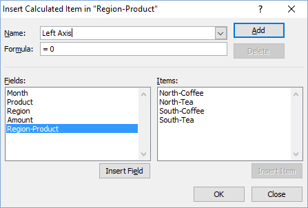
How to Concatenate Values of Pivot Table - Basic Excel Tutorial Click insert Pivot table, on the open window select the fields you want for your Pivot table. Once you select the desired fields, go to Analyze Menu. Under calculations, choose fields, Items & Sets tab then click on calculated fields. Enter the values and click ok. Your PivotTable will display the total of combined units and price. Like this:

Excel Help: Simple method to make Pivot table

Design the layout and format of a PivotTable On the Options tab, in the PivotTable group, click Options. In the PivotTable Options dialog box, click the Layout & Format tab, and then under Layout, select or clear the Merge and center cells with labels check box. Note: You cannot use the Merge Cells check box under the Alignment tab in a PivotTable.

How-to Make an Excel Stacked Column Pivot Chart with a Secondary Axis - Excel Dashboard Templates

Excel 2016 Pivot table Row and Column Labels - Microsoft Community In Excel 2016 I've found when I create a pivot table it unhelpfully shows 'Row Labels' and 'Column Labels' instead of my field names, although in the top left cell it says 'Count of' and then inserts the correct field name. Years ago when I last used Excel it automatically put the field names in all three heading cells.

How to Insert an Excel Pivot Table - YouTube

How to Move Excel Pivot Table Labels Quick Tricks To move a pivot table label to a different position in the list, you can use commands in the right-click menu: Right-click on the label that you want to move Click the Move command Click one of the Move subcommands, such as Move [item name] Up The existing labels shift down, and the moved label takes its new position. Type Over Another Label

Design your Pivot Table in Excel | Excel in Excel

Pivot table row labels side by side - Excel Tutorials You can copy the following table and paste it into your worksheet as Match Destination Formatting. Now, let's create a pivot table ( Insert >> Tables >> Pivot Table) and check all the values in Pivot Table Fields. Fields should look like this. Right-click inside a pivot table and choose PivotTable Options…. Check data as shown on the image below.

Excel Pivot Table Report - Sort Data in Row & Column Labels & in Values Area, use Custom Lists

Excel tutorial: How to rename fields in a pivot table Either right-click on the field and choose Value field settings, or click Field Settings on the Options Tab of the PivotTable Tools ribbon. Here, you can see the original field name. In contrast to value fields, Row and Column label field names will be identical to the name in the field list. In fact, they are linked, as we'll see in a minute.

Share :